Automatic reduction of spectral
data
|
SpcAudace |
![]()
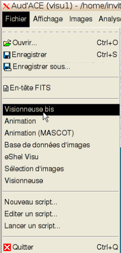
1. Configuration and preliminary tunings in Audela
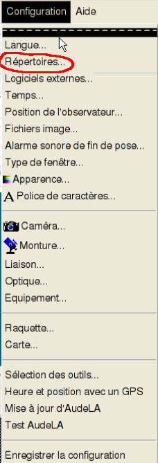
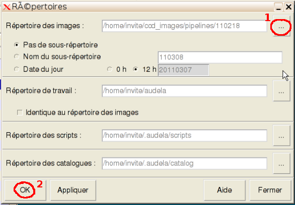
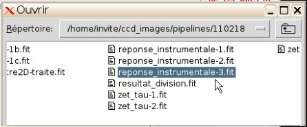
Beware:all the data to be processed ( 2D spectral images (including those associated with the calibration lamps), darks, flats, darks associated with the flats, offsets (if relevant)) must be located in this directory.
![]()
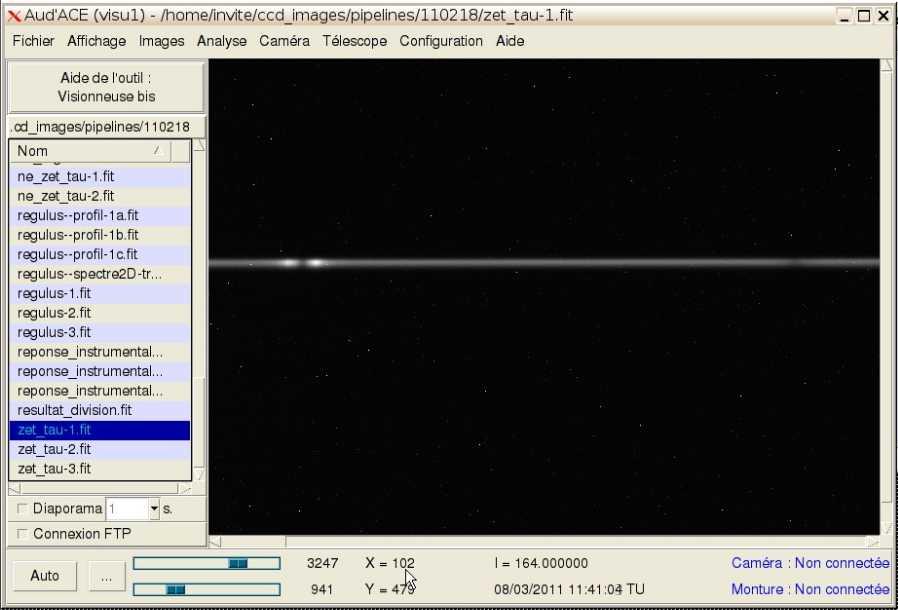
2. Launch the pipeline dedicated to the automatic reduction of spectral data
We process here the spectral data acquired on zeta Tau, a bright Be star in the Taurus constellation.
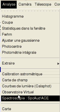
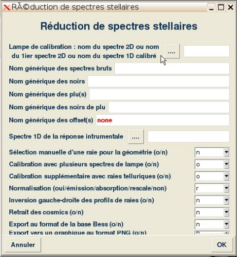
From the Pipelines menu, click on "Pipeline 2a". The pipeline number 2a window shows up:
![]()
![]()
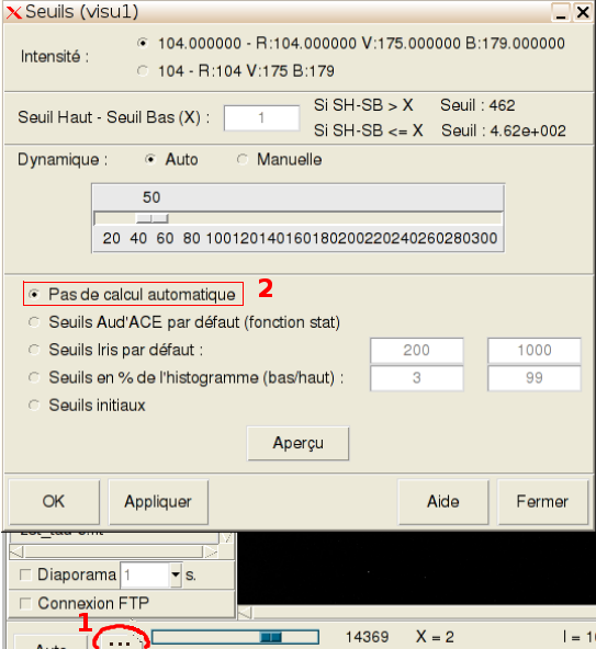
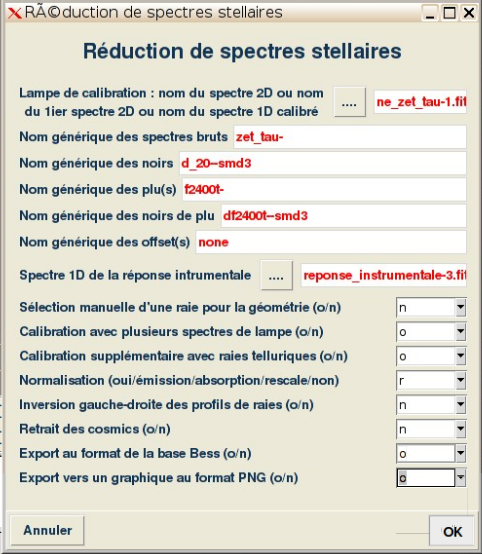
4. Computational options
The remaining of the form concerns different options to be specified for the computation. The default settings are appropriate for most of the cases you will encounter. They rarely have to be changed, especially for high resolution spectroscopy. Thus the information in this section is mainly given for sake of completeness.
Click on "OK" to lauch spectral data reduction.
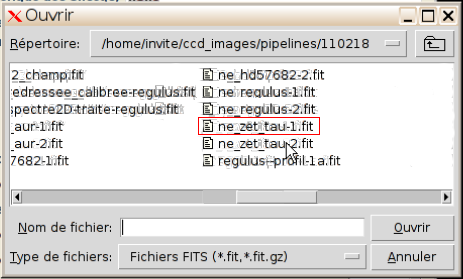
The pipeline starts with the determination of the smilex correction that makes the lines in the calibration image as straight as possible.
Next, it preprocesses the raw images and after that, it opens a new window dedicated to the spectal calibration.
![]()
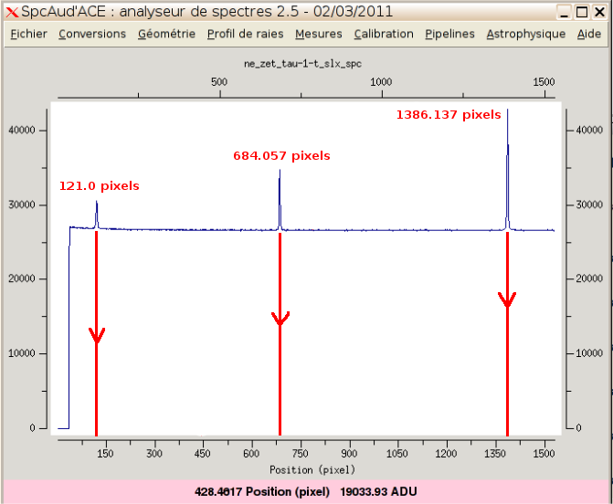
Next click on "OK" to launch the last computations. The pipeline then completes spectral data reduction and produces profiles up to level 2b.At this stage, the profile computed from the calibration image is displayed in the SpcAudace window:
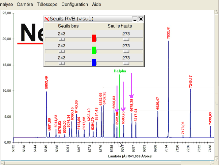
To help the user, an annotated image of the neon spectrum is displayed in Audela's Visu 1 window:
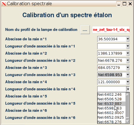
It is then straightforward to match the lines in the uncalibrated profile with those of the neon lamp. In our example, three lines, with almost equal separation and with increasing intensities are to be found. You will recognize lines with wavelenghts 6532.93 A, 6598.95 A et 6678.28 A. Matching the main lines in the profile and neon wavelengths is achieved through the calibration window:
By clicking on the downward pointing arrow, rignt to the empty boxes, on the lines "Longueur d'onde associée à la raie n° X" (wavelength associated with line number X), you can span the wavelengths specific of each chemical element. "NeI" corresponds to neon. Using the accurate wavelengths available from the library allows an accurate calibration.
If one of the lines in the profile is not detected, it is possible to enter its location (in pixels) through the keyboard.
It is mandatory to keep the wavelength boxes associated with lines that SpcAudace may have erroneously detected empty. These lines will then be ignored.
In our example, only lines with coordinates 1386.137, 684.057 and 121.0 pixels are to be paired with wavelengths. The pixel coordinates may show slight variations for different runs of the pipeline. This stems from slight variations in the geometrical corrections since the pipeline is adaptative according to the situation it meets.
The pixel coordinate to wavelength map (calibration map) is modeled by a low degree polynomial. Its degree depends on how many lines you have selected:
- with two rays (minimum required), first degree polynomial;
- with three rays, second degree polynomial;
- with four rays or more, third degree polynomial;
The parameters that define the calibration map are stored in the FITS header:
- coefficients describing the polynomial : SPC_A, SPC_B, SPC_C et SPC_D for λ=a+b*x+c*x2+d*x3.
- in case of a profile regularly sampled in wavelength (linear calibration map): CRVAL1 et CDELT1 for λ=CRVAL1+CDELT1*x.
with x defined by: x=pixel number-CRPIX1 (CRPIX1 is the FITS keyword defining the reference pixel).
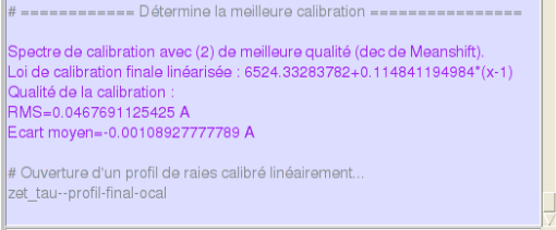
In the end, the pipeline produces profiles that are regularly sampled in wavelength: an interpolation is then required unless the polynomial was first degree (this interpolation is inproperly called "linéarisation de la loi de calibration"). This allows these profiles to be read by all astromical softwares.
![]()
You can inspect the progress in the pipeline computations through Audela's console. The different steps of these computations are:
- Preprocess of raw images.
- Geometrical corrections:
- Correction for the smilex.
- Correction for tilt.
- Vertical registration.
- Horizontal registration (whenever 2 calibration images are available).
- Stack (summation) of the so-corrected images.
- Sky background estimation and subtraction.
- Binning of columns to produce a spectral profile.
- Application of the computed calibration map to the profile of the star (here zet Tau)
- Correction for the instrumental response.
- Regular resampling (in wavelength) of the profile.
- Display of the final profile in the SpcAudace window.
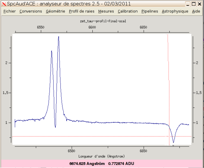
Finally, the spectral profile with level 2b of zeta Tau is displayed:
Final products are stored in the working directory. You may find the following files, depending on options selected in the pipeline:
- zet_tau--profil-final-ocal: lines profil of the star with all options applied, in our example, continuum is rescaled and it is calibrated with telluric lines (-ocal suffix);
- zet_tau--profil-2b-ocal: same file as described;
- zet_tau--profil-2b: lines profil with continuum rescaled;
- zet_tau--profil-1c: lines profil corrected from instrumental response;
- zet_tau--profil-1b: lines profil with wavelength calibration made with the spectral lamp;
- zet_tau--profil-1a: uncalibrated lines profil;
- zet_tau--spectre2D: 2D spectrum coming from the 32 bit summation of the 3 preprocessed spectra of zet Tau and corrected from geometrical deformations.
![]()
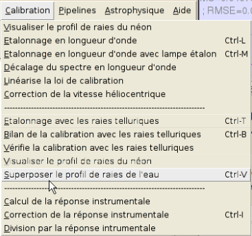
7. Quality check of the wavelength calibration
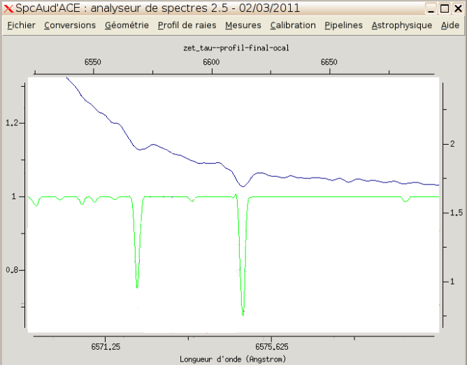
You can easily check this quality by superimposing the telluric lines with the computed profile: from the Calibration menu, click on "Superposer le profil de raies de l'eau" :
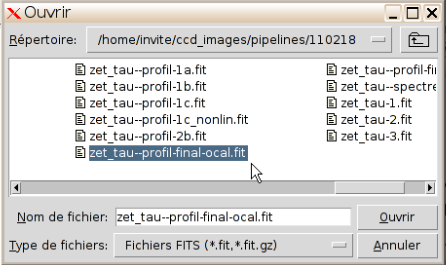
You then have to specify the name of the file containing the star profile:
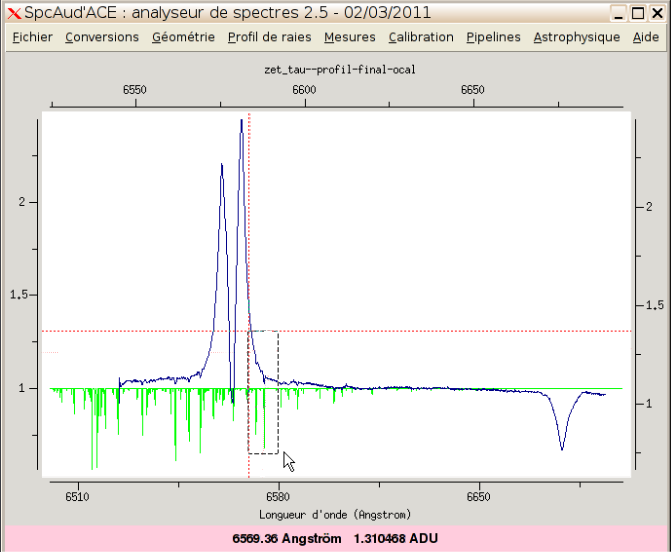
The intensity of profile of the telluric lines is automatically adapted so as to match the intensity of the stellar profile:
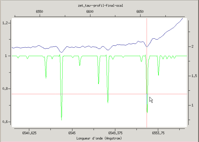
You can zoom on the lines right to the Halpha line for a more accurate inspection:
To come back to the no zoom display, right click on the SpcAudace window. In the same way, you can inspect the area left to the Halpha line:
There is good match between telluric lines and absorption lines in the stellar profile, an indicator of a correct calibration.
Besides, numeric indicators concerning the quality of the calibration are computed. The results are stored the FITS header through the keywords below:
- SPC_RMSO : estimate of the RMS mismatch between telluric lines and the corresponding lines observed in the stellar spectrum; this estimate depends on several factors such as the signal to noise ratio for instance.
- SPC_MDEC : the average mismatch, indicator of a possible global shift using telluric lines.
- SPC_CALO : name of the method used to improve calibration using telluric lines.
- SPC_RESP : spectral resolution estimated from the calibration image.
![]()
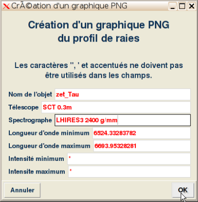
8. Export an image in PNG format
At the end of the pipeline, the window dedicated to export an image in PNG format shows up, if asked by the user when filling the first form. You just have to fill the form unless the information can be found in the FITS header.
Usually, just the name of the spectrograph and the name of the star are to be specified:
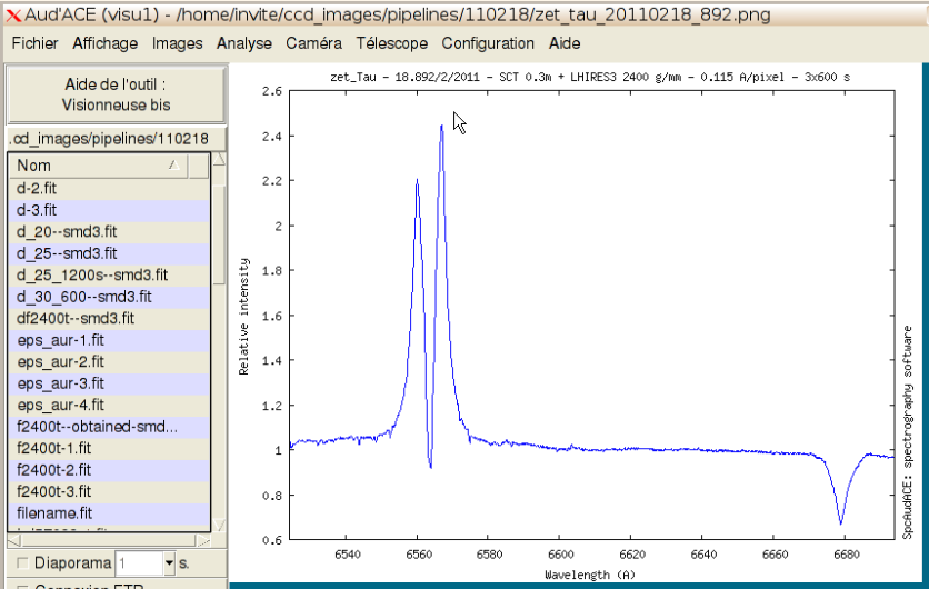
The constructed PNG file is displayed in Audela's Visu 1 window, with the title matching the information given above.
Afterwards, another window shows up, if asked by the user when filling the first form.
![]()
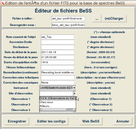
Once the quality of the calibration has been checked and if no anomaly is revealed, you can submit the profile to the BeSS database and thus participate in a collaboration between professionnals and amateurs focused on the observation of Be stars. You just have to fill the form below:
For that you must :
- Give the correct name of the star (e.g.: alp Gem, del Sco) : "zet Tau".
- Specify your instrumentation by scrolling the dedicated menu. However, your instrumentation has first to be registered in your Bess account.
- Choose the observation site still by scrolling the dedicated menu. Again, this site has first to be registered in your Bess account.
- Give the observer's name provided that this name is registered in your Bess account.
For a first use of this export window, you must edit the different lines using the button "Editer les configs".
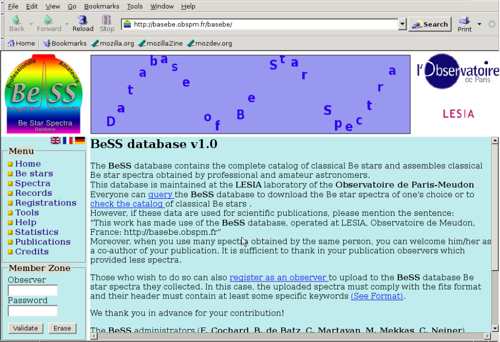
Once the different items have been completed, click on "enregister les modifications". The exported spectrum appears with the prefix "bess_". You can now submit this spectrum to the BeSS web site: click on "Web BeSS". The Bess web page then appears in your web browser:
Just enter your identifier and password and upload your spectrum.
The processing is completed. You can proceed to the data associated with the next object!