Use of Pipeline 1 for the computation of the instrumental response

SpcAudace

 1. Configuration and preliminary tunings in Audela

1. Specify the directory containing the data to be processed :
   In the Configuration menu, select Répertoires.

   

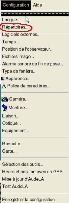
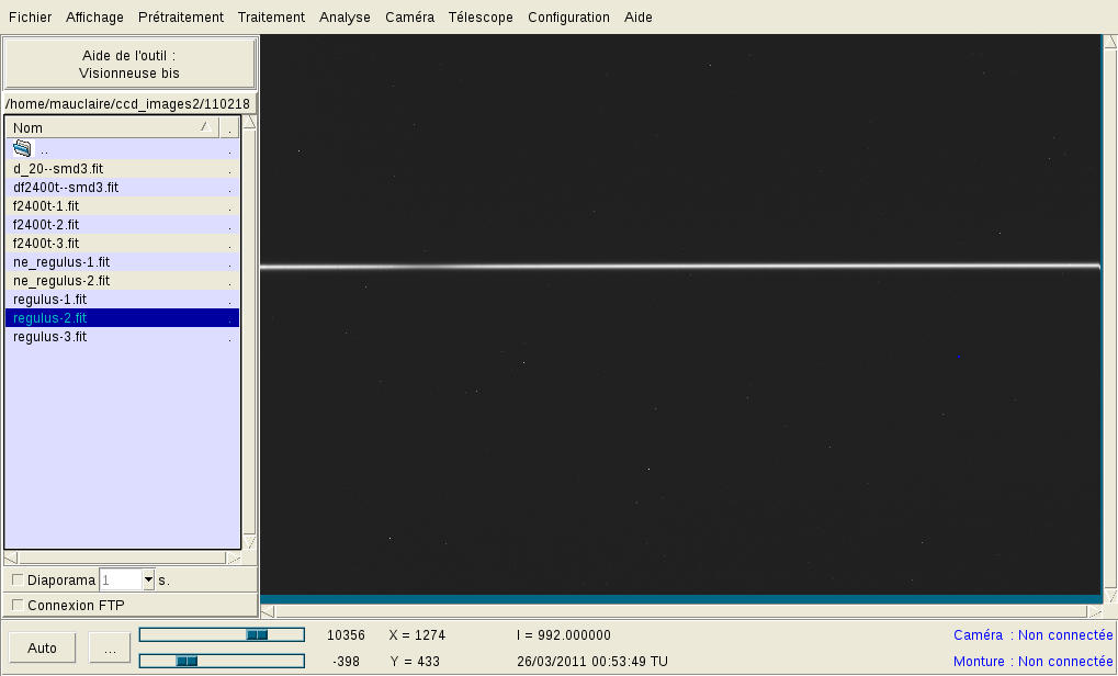
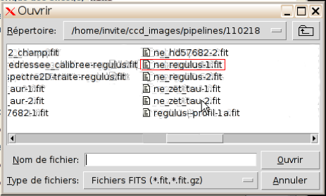
   Use "..." to reach the desired directory.

   

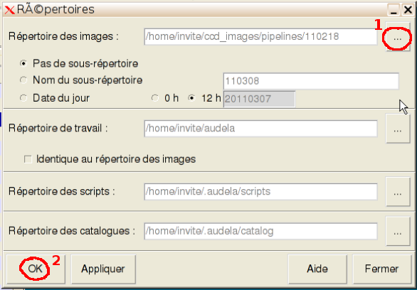
   Beware: all the data to be processed ( 2D spectral images (including those associated with the calibration lamps), darks, flats, darks associated with the flats, offsets (if relevant)) must be located in this directory.

2. Use Audela's "Visionneuse bis" to have  an overiew of the concerned files:
   

   

   By clicking on a file, it will be displayed. You can also use the keyboard Up and Down buttons to navigate from one file to its neighbours.

3. Tune the display thresholds:
   The goal is to make visible in the same time the telluric lines within the continuum as well as possible cosmics.

   

   
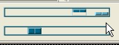
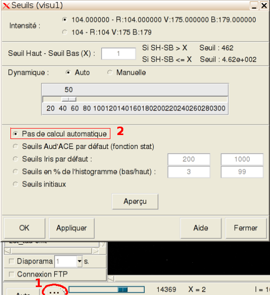
   It is preferable to uncheck the automatic threshold adjustment. In this end, click on the "..." button, just left to the cursors used for the tuning of the thresholds:

   

4. Check the raw spectral images and eliminate images showing poor quality data:
   

   

 2. Launch the pipeline dedicated to the computation of the instrumental response

Using the spectrum of the 3 proposed reference stars (Regulus, Altair and Castor) allows a straightforward computation of the instrumental response. This is illustrated below, using the spectrum of Regulus.

1. Launch SpcAudace :
   This is achieved through the Analyse menu in Audela.

   

2. Launch pipeline number 1 for the computation of the instrumental response:

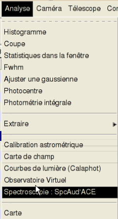
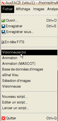
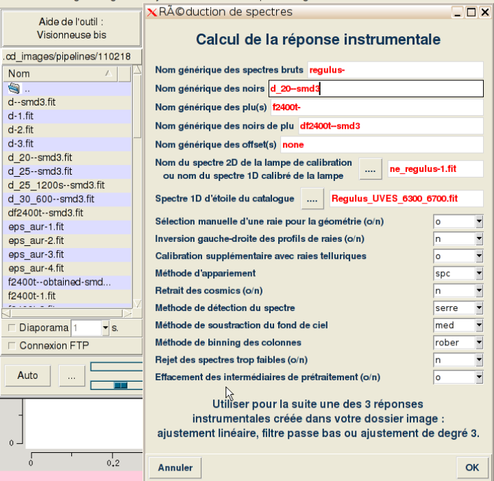
   From the Pipelines menu, click on "Pipeline 1". The pipeline number 1 window shows up:

   

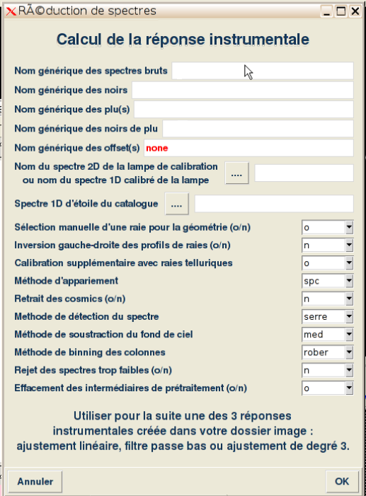
 3. Fill the associated form

1. Unprocessed files' generic name (genenic name for raw spectra):
   Since Regulus has been chosen as reference star for the computation of the instrumental response, the names of the acquisition images for this target are: regulus-1.fit, regulus-2.fit and regulus-3.fit. Thus the generic name to be specified is: "regulus-".
2. Dark's generic name (genenic name for darks):
   In the same way, we specify the generic name, here d2400t-, for the raw dark images.However, if a master dark has already been computed, we just have to give its name, for instance, "d2400t--smd3.fit". 
3. Flat's generic name (generic name for flats):
   Specify the generic name for the raw images.
4. Flat's dark generic name (generic name for the darks to be applied to flats):
   Again, we can either specify the generic name for the raw images or the name of the master image: "df2400t--smd3".
5. Offset's generic name (generic name for bias images):
   If bias images are to be used (that is in case of different exposure durations for the images and the corresponding darks), enter the bias generic name. Otherwise, keep "none".
6. 2D calibration file's name or calibration lines profile's name (name of the 2D spectrum of the calibration images):
   In order to calibrate stellar (or other astronomical object) spectra, you have taken calibration images (images of a calibration lamp, neon in general) before and after the acquisition of the spectral images. By clicking on "....", select the first of the calibration image you have taken, here, in our example, "ne_regulus-1.fit". In case only one calibration image is available, select it. However, it is highly recommended to
   take several calibration images, at least one just before capturing the spectrum of an object and one just after, if a long (more than 15 minutes) exposure is required. Indeed the calibration images are used, not only for the calibration, but also for the horizontal registration of the different images

   

7. Catalogue star's lines profil (1D catalogue spectrum of the reference star):
   Clicking on "..." opens a window that shows the catalogue spectral profiles of different stars. These profiles are calibrated. Select the one corresponding to the reference star you have captured. SpcAudace catalogue contains UVES spectra of Altair, Castor and Regulus. Depending on the spectral window covered by your instrumentation, you may be led to choose between the 6000-7000 A or the 6300-6700 A band. With our KAF1600 sensor and a 2400 g/mm grating centered on Hα, we choose : "Regulus-UVES-6300-6700.fit".

   

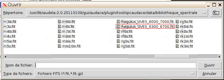
 4. Computational options

The remaining of the form concerns different options to be specified for the computation. The default settings are appropriate for most of the cases you will encounter. They rarely have to be changed, especially for high resolution spectroscopy. Thus the information in this section is mainly given for sake of completeness.

• Sélection manuelle d'une raie pour la géométrie (manual selection of a ray for geometrical corrections):
  o(oui=yes) ou n(non=no) depending on whether you want or not an automatic detection of the central line in the calibration image. The selected line will be the one used for the estimation of the smilex in the spectra.
• Inversion gauche-droite des profils (left-right inversion):
  The convention is to have the blue side at the left of the spectra. Your data fulfill this convention if your camera is properly mounted on the spectrograph. If not, choose "o" (oui) in order to invert left and right. The default setting corresponds to data that fulfill the convention.
• Calibration supplémentaire avec les raies telluriques (use telluric lines to improve the calibration):
  If you have enough spectral resolution, you may expect telluric lines to be observable. Using these lines is likely to improve the calibration. If you want to catch this opportunity select option "o" (oui/yes).
• Méthode d'appariement (technique used for vertical registration of the images) :
  Three options are proposed for this registration: "spc", "reg" et "n", for vertical, stellar or no registation, respectively. The "spc" option is the one that usually works best.
• Retrait des cosmics (cosmics removal):
  If your raw images are contaminated by many cosmics, you can attempt at removing them by choosing option "o". But the drawback is a slight degradation of the signal to noise ratio. Alternatively, you can apply the procedure spc_scar to the profile you will obtain. This procedure modifies the profile only locally.
• Méthode de détection du spectre (method used for spectrum detection):
  The pipeline needs to identify the area where spectral information is localized as opposed to the sky background. we propose two methods depending whether you want a narrow ("serre") or a broad ("large") area. Usually the option is to be preferred. However if you deal with poor signal to noise data, you may be led to use the "large" option.
• Méthode de soustraction du fond de ciel (method used for sky background subtraction):
  The sky background is to be substracted to the pixels located in the area where spectral information is localized (spectral area). The sky background is assumed to be a constant whose value has to be estimated. Several methods are proposed for this estimation.
  
  • "med": the value is obtained by taking the average of two estimates; these estimates are obtained by computing the median of the pixels within one band above the spectral area and one below; the vertical width of these bands is one of the spectral area.
  • "moy" : same, but the average is used in replacement of the median.
  • "moy2" : same, but we use here a weighted average.
  • "sup" : the estimation does not consider here the area below the spectral area.
  • "inf" : the estimation does not consider here the area below the spectral area.
  • "back" : the estimation uses a filter with kernel background.
  • "none" : the estimated value is zero.

  The method "med" gives best results in most cases.

• Méthode de binning des colonnes (method for column binning):
  The profile is obtaine by a column binning. Three methods are proposed:
  
  • "add": mere binning.
  • "rober": binning based on a weighted average including a rejection of outliers.
  • "horn": Horner method, not yet implemented.

  Method "rober" turns out to be the most effective.

• Rejet des spectres trop faibles (weak spectra rejection):
  Raw images showing a poor signal to noise ratio (this is likely to occur in case of a sudden cloud or in the case of problem with autoguiding) are not taken into account if you have chosen option "o".
• Effacement des intermédiaires de prétraitement (removal of intermediate files):
  At different stage of the processing intermediate files are created. Since they are in general useless, they are removed at the end of the pipeline (option "o"). However, if you need them for analysis, just select option "n".

Click on "OK" pour launch the pipeline.
It starts with a smilex correction of the lines in the calibration image. Next, it preprocesses the raw images and after that, it opens a new window dedicated to the spectal calibration. This is the only stage where the user has to provide additional information.

 5. Spectral calibration

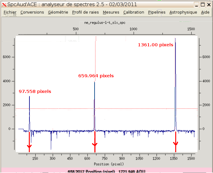
At this stage, the profile computed from the calibration images is displayed in the SpcAudace window:

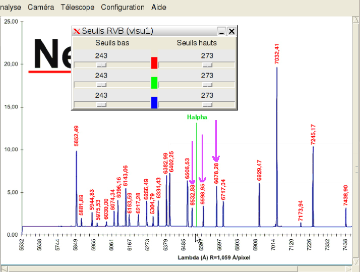
However this profile is not calibrated in wavelength. To achieve spectral calibration, several lines in this profile are to be matched with the wavelength of the lines in the (neon in the case of a LHIRES3 spectrograph) calibration lamp. To user is implied for specifying this match. To help the user in this task, an annotated image of the neon spectrum is displayed in Audela's Visu 1 window:

It is then straightforward to match the lines in the uncalibrated profile with those of the neon lamp. In our example, three lines, with almost equal separation and with increasing intensities are to be found. You will recognize lines with wavelenghts 6532.93 A, 6598.95 A et 6678.28 A.

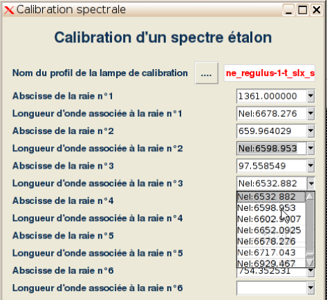
Matching the main lines in the profile, which are automatically detected by SpcAudace, and neon wavelengths is achieved through the calibration window:

By clicking on the downward pointing arrow, rignt to the empty boxes, on the lines "Longueur d'onde associée à la raie n° X" (wavelength associated with line number X), you can span the wavelengths specific of each chemichal element. "NeI" corresponds to neon. Using the accurate wavelengths available from the library allows an accurate calibration.

If one of the lines in the profile is not detected, it is possible to enter its location (in pixels) through the keyboard: just place the mouse in the center of the line and look at the value displayed below the image. In order to keep accuracy it is highly recommended to zoom the SpcAudace window.

It is mandatory to keep the wavelength boxes associated with lines that SpcAudace may have erroneously detected empty. These lines will then be ignored.

In our example, only lines with coordinates 1361.0, 659.96 and 97.558 pixels are paired with wavelengths. The pixel coordinates may show slight variations for different runs of the pipeline. This stems from slight variations in the geometrical corrections since the pipeline is adaptative according to how the spectrograph is blended.

The pixel coordinate to wavelength map (calibration map) is modeled by a low degree polynomial. Its degree depends on how many lines you have selected:

• with two rays (minimum required), first degree polynomial;
• with three rays, second degree polynomial;
• with four rays or more, third degree polynomial;

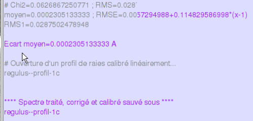
In the end, the pipeline produces profiles that are regularly sampled in wavelength: an interpolation is then required unless the polynomial was first degree (this interpolation is inproperly called "linéarisation de la loi de calibration"). This allows these profiles to be read by all astromical softwares.

Next click on "OK" to launch the last computations. The pipeline then completes spectral data reduction and produces profiles up to level 1c. The pipeline also displays three different possible instrumental responses.

 6. The pipeline run

You can inspect the progress in the pipeline computations through Audela's console. The different steps of these computations are:

1. Preprocess of raw images. This includes the computation of a master dark and of a master flat. The master dark is obtained by selecting the median value for each pixel.
2. Geometrical corrections:
   
   1. Correction for the smilex.
   2. Correction for tilt.
   3. Vertical registration.
   4. Horizontal registration (whenever 2 calibration images are available).
3. Stack (summation) of the so-corrected images.
4. Sky background estimation and subtraction.
5. Binning of columns to produce a spectral profile.
6. Application of the computed calibration map to the profile of the reference star (here Regulus).
7. Estimation of 3 possible instrumental responses.
8. Correction for the instrumental response using the default instrumental response.
9. Regular resampling (in wavelength) of the profile .
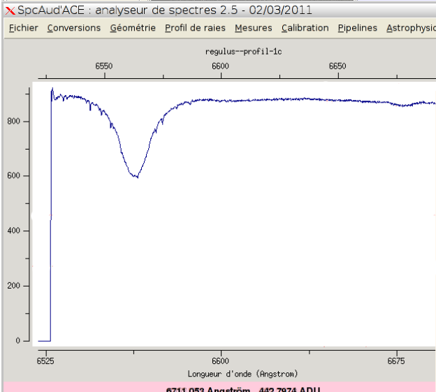
10. Display of the final profile in the SpcAudace window.

Display of the final (level 1c) profile in the SpcAudace window.

 7. Choosing the instrumental response

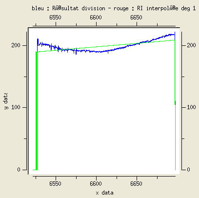
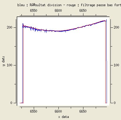
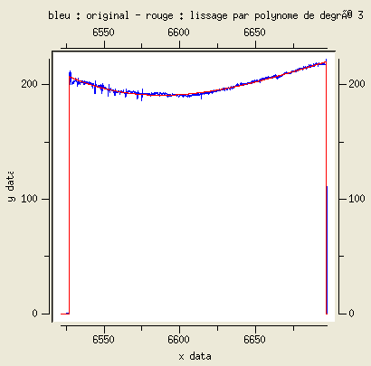
The 3 computed instrumental responses are saved in files: reponse_instrumentale-1.fit, reponse_instrumentale-2.fit and  reponse_instrumentale-3.fit. These instrumental responses are obtained by applying different filters to the result of the division of the level 1b profile by the catalogue profile of the star.
The pipeline displays these 3 instrumental responses (in red) superimposed with the result of the division (in blue):

reponse_instrumentale-1.fit	reponse_instrumentale-2.fit	reponse_instrumentale-3.fit

reponse_instrumentale-3 best matches the result of the division while keeping very smooth. This the most frequent situation and this instrumental response has been used (default setting) for the computation of the level 1c profile of Regulus displayed above. This instrumental response is the one to be used for correcting the spectral data acquired with the same instrumentation.

==> See tutorial for Pipeline 2a for the reduction of stellar high resolution spectral data.